Take a language model apart.
One experiment at a time.
The slow, visual version of the repo — no walls of text; every idea is something you poke, drag, or toggle. Move with the tabs on the left, the Prev / Next buttons, or the ← → keys. Each tab is one experiment and stands on its own.
Tabs are ordered for learning, not by folder number — so related experiments sit together (the repo № on each tab still points back to its folder).
The induction circuit: find it, break it
The foundational experiment. Force the model to copy, watch where it succeeds, then delete the heads that do the copying and watch the ability vanish — a causal proof, in three moves.
① The setup — a trick that forces the model to copy
Feed the model a list of random tokens, then the exact same list again. The second time, the only way to predict what's next is to look back and copy.
② The cliff — and switching it off
Plot how surprised the model is at every position. Watch it fall off a cliff when copy 2 begins — then hit ablate and watch the cliff refill.
③ What an induction head actually does
An attention head lets each token "look back." An induction head has one habit: find where this token appeared before, then look at whatever came right after it.
go deeper — why random tokens, and what's the "induction score"?
Random tokens carry no grammar or facts to lean on — the only signal is the repetition. So nailing copy 2 must be in-context learning, not memorized trivia. Ablate = a forward hook on blocks.{L}.attn.hook_z zeroes just those heads' output; if the cliff refills, they caused the behaviour (on gpt2 the jump is 36×). The induction score is each head's average attention on the look-back-and-shift diagonal — plot it per (layer, head) and the dots are the induction heads (gpt2 has a couple; Qwen3.5-4B stacks 34).
"But maybe any heads matter?"
Fair challenge. So ablate the same number of randomly chosen heads instead, 10 times. If random ablations barely hurt while the induction heads devastate — the damage is specific to the circuit, not to losing some heads.
go deeper — what's a "σ" (sigma)?
σ (standard deviation) measures the spread of the 10 random trials. Saying induction ablation is "102σ above the random mean" (Pythia-1.4B) means: on the bell curve of random damage, the induction result is absurdly, off-the-chart worse — astronomically unlikely to be a coincidence. That's how you turn "it looks important" into a number.
The circuit has two halves
The induction head can only copy "what came after last time" if some earlier head already tagged each token with who came before it. That upstream helper is the previous-token head. Cut it, and the induction head goes blind — without touching the induction head at all.
Next tab (Layer knockout) chases the same upstream signal into the hybrid models, where the previous-token head hides in a surprising place.
Follow the signal upstream
Some layers can't be scored for induction (the hybrid models' linear-attention layers show no attention pattern) — but they can still be knocked out. Remove one attention layer at a time, re-measure the induction heads, and read off which layers they secretly depend on.
go deeper — the "just-in-time shift register"
In the hybrid Qwen3.5 models there were no previous-token heads in the normal attention layers (tab 3 couldn't find them). This lesion study shows why: the upstream signal lives in the linear-attention layers, and specifically the one directly before each induction layer — L14 feeds L15, L10 feeds L11 — acting as a local shift register that delivers "the previous token" exactly when it's needed. gpt2 validates the method: layer 0 is foundational (everything builds on it), and its previous-token signal is spread thinly across several mild layers. (Non-critical layers shown near baseline; the deep dips are the measured ones.)
The Hydra: cut a head, a backup wakes up
Ablate the main induction heads and re-score every remaining head inside the broken model. In some models, heads that looked useless suddenly step up to do the job — backups that were invisible until needed. Cut one head, two grow back.
Is this self-repair real, or an artifact of how we ablate? The next two tabs answer that — first mean-ablation, then faithful patching.
Zeros, or the average?
"Delete a head's output" hides a choice: what do you replace it with? Zeros are simplest but off-distribution — the model never saw an all-zero activation in training, so it may overreact. Replacing with the head's average keeps a realistic size while still deleting the information.
go deeper — why this matters
If zeroing and mean-ablation disagree, some of the "damage" (or self-repair) is really a distribution shock, not the model's true behaviour. On Qwen3-1.7B they agree (2.9× ≈ 3.0×), so its tiny damage is genuine redundancy — the Hydra from tab 5 is real, not a LayerNorm artifact. On gpt2/Pythia, zeroing overstates the damage ~1.5×; every conclusion survives the calibration, but it's worth knowing which number is honest.
The gold-standard null: patching
The most faithful ablation replaces a head's output with a real activation from a matched control run — same first copy, but a fresh, non-repeating second half. Same-sized, in-distribution, zero shock. It surgically nulls only the induction region.
Because attention is causal and the first halves match, patching is a no-op on copy 1 and only changes the copy-2 (induction) predictions.
go deeper — the verdict on the Hydra
The payoff: on Qwen3-1.7B, faithful patching recruits the same backups as zero-ablation (L21H9, L18H4, L8H5), so the self-repair is a genuine property of the network, not a zeroing artifact. But the damage-magnitude ordering (zero vs mean vs patch) turns out to be model-dependent — there is no universal ranking. The robust cross-model claim isn't "which is biggest," it's that patch and zero agree on which backups exist.
Watch the circuit be born
Circuits aren't there at the start — they snap into existence during training. Drag through 14 real Pythia-160m checkpoints and watch the induction score sit near zero… then ignite between steps 512 and 1000.
go deeper — the built-in control
See the flat grey line? That's copy-1 surprise — the un-copyable half. It stays pinned at ~13 the entire run. If the drop were just "the model getting generally better," copy-1 would fall too. It doesn't. Only the copyable half improves, and only after the circuit ignites — the control that makes the story airtight.
Grow one yourself — the data decides
This experiment trains a tiny model from scratch, three times, changing only the data mix. Story-only data never grows the circuit. Add the right pressure and it ignites in a single 8-million-token window. The recipe matters, not just the size.
go deeper — why doesn't TinyStories alone work?
Interesting split: the upstream half (prev-token heads) forms for free on almost any text — it reached 0.57 even on stories alone. But composition — wiring that upstream signal into a copying circuit — only happens when the data rewards copying. The synthetic repeated-block rows are that reward: the only way to predict them is to copy. 85% real text + 15% synthetic ignited; 30% wikitext with no synthetic stalled at 0.065 after 445M tokens. The circuit needs a reason to exist.
Same tools, new question: refusal
A chat model's decision to refuse turns out to live along a single direction in its activations. Slide it: remove the direction and a harmful prompt gets answered; add it and a harmless prompt gets refused. A clean double-dissociation.
go deeper — how do you "find a direction"?
Run a batch of harmful prompts and a batch of harmless ones. Average each group's residual-stream activation at the last token, and subtract. That difference vector is the refusal direction (best layer by separation — here layer 21 of Qwen2.5-1.5B). "Remove it" = project it out of every layer; "add it" = add it in. Directions are the feature-level cousin of heads — exactly where mech-interp heads next (sparse autoencoders find thousands of them). This same direction is the tool used in the next two tabs.
Did "unlearning" erase it? — the generation test
Companies "unlearn" facts for safety. First test: does the model still generate the forgotten answer? Measured by ROUGE-L overlap with the truth on five TOFU-unlearned checkpoints, against a floor (never learned it) and a ceiling (learned it normally).
Generation only sees the model's top choice. The next tab asks a sharper question — the probability it assigns the true answer — and the story changes.
The same question, asked by probability
"Does the model know X" is really about the probability it puts on the true answer — not just its greedy guess. Rerun with that metric and the murky result turns sharp: one method was only hiding the knowledge, and one intervention brings it back.
go deeper — why this matters for alignment
"We unlearned it" is a safety claim, and this shows a safety claim can be an artifact of the metric. NPO looks fully forgotten under generation (tab 11), but its answer probability is only suppressed — ablating the refusal direction lifts it 4× back above the floor. GradDiff genuinely forgot; RMU barely forgot on Q&A at all. Same word — "unlearned" — three different realities. Building tools and evals that catch this is a real contribution to safe, trustworthy AI.
Everything above, as a 3D replay
The same runs, staged as a game of Battleship: copy 1 is the fleet, copy 2 is the targeting board, and a wall of attention heads sits between them. Attention is drawn as light; every prediction drops a peg — green hit, red miss.
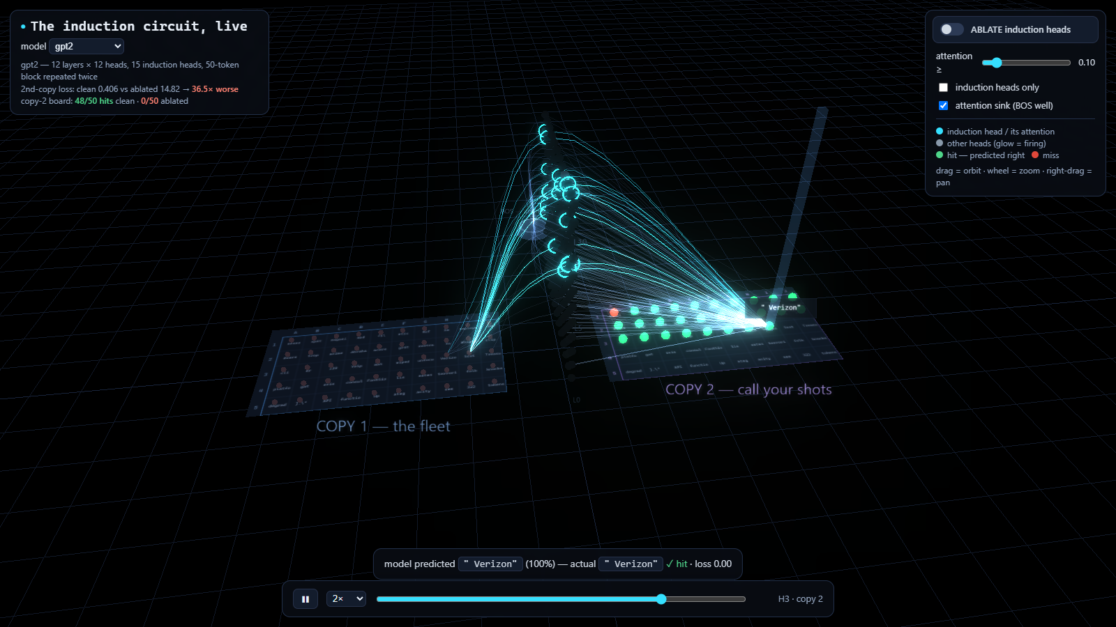
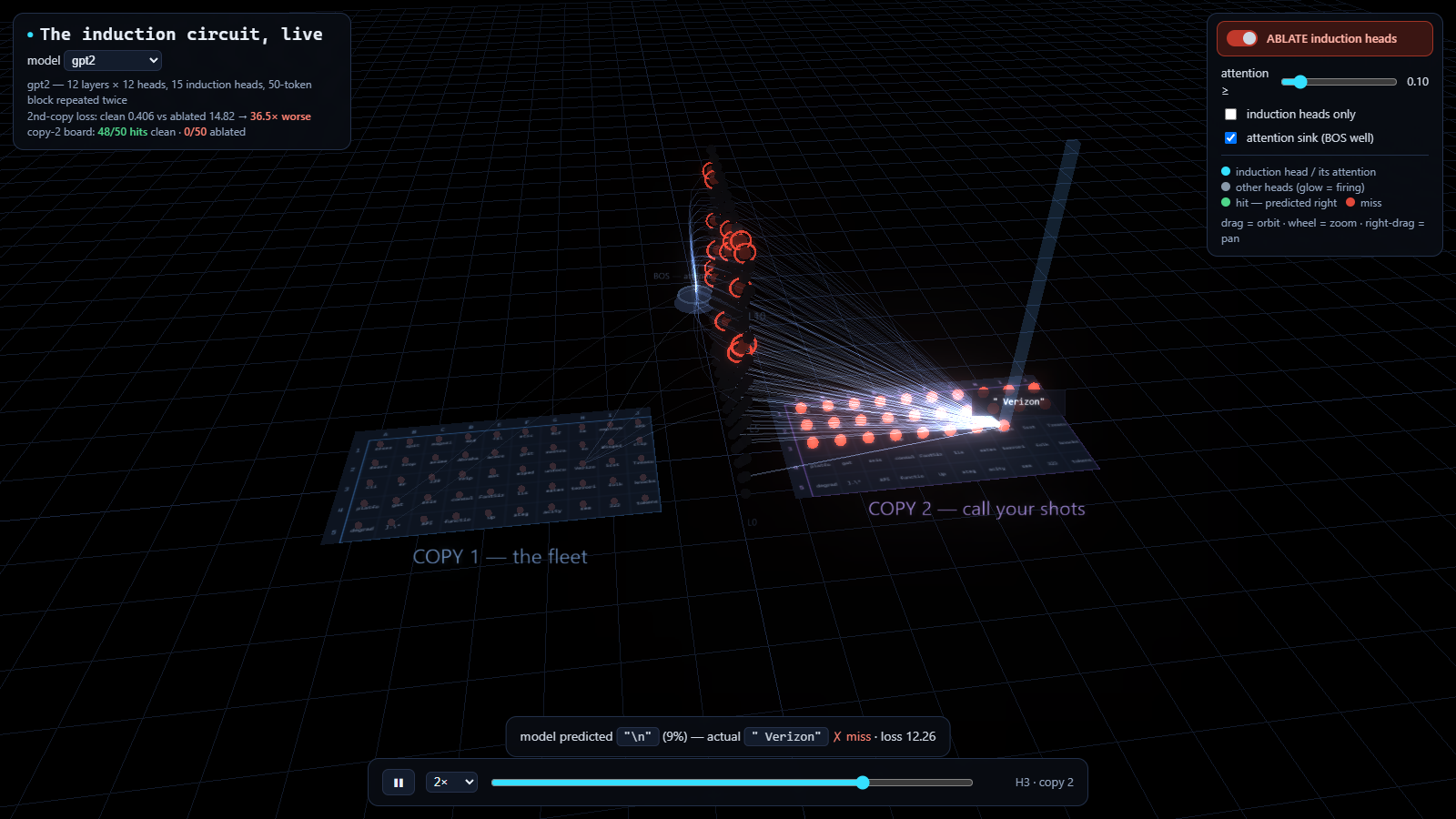
Six scenes — the induction circuit, the refusal direction (tab 10), the training-time birth (tab 8), the unlearning gauge (tabs 11–12), the SAE dictionary (tabs 18–20), and the attribution graphs (tab 25) — all on the same stage.
In the SAE scene the wall of heads becomes a wall of dictionary features: scrub a prompt and watch feature #2673 light up on harmful requests but stay dark on harmless ones, flip the diet to see the safety corner empty out (tab 18) or fill in (tab 19), then ablate it and watch the harmful board flip from REFUSED to answered (tab 20).
In the attribution graph scene, tab 25's circuits replay as edges firing: the prompt's token cards ignite, pulses sweep up the edges layer by layer through the feature nodes, and the answer logit lights up last. A selector flips between the two traced prompts — dallas (the capital-city chain) and ioi (who gets the drink).
Too many ideas, too few dials
A feature is a direction — a concept stored as a push on the model's internal dials. The catch: models track more features than they have dials. When features rarely fire together, the model crams them in by letting them overlap and take turns. That's superposition — and it's why a single neuron lights up for many unrelated things.
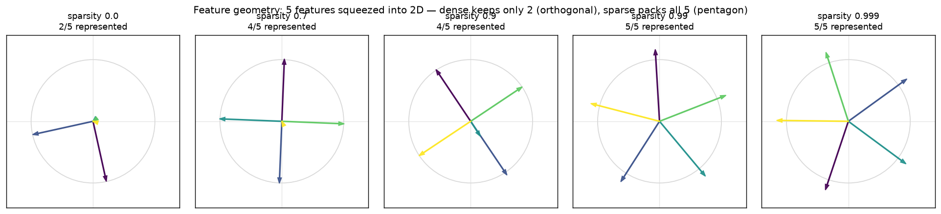
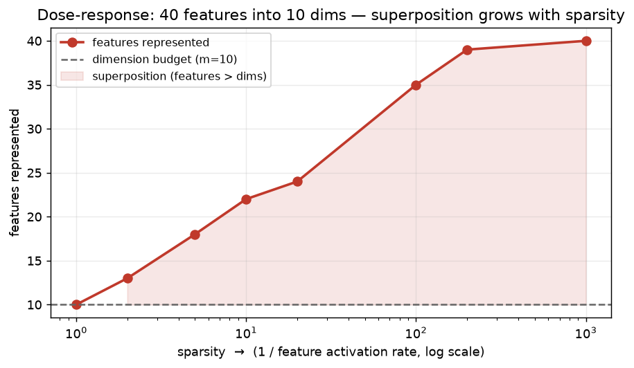
go deeper — the honest catch
The toy is a bottleneck autoencoder trained to reconstruct sparse synthetic features through too few dimensions. With equal feature importance it spreads itself thin (a degenerate smear); giving features decaying importance makes it cleanly keep the important ones and drop the rest — dense keeps exactly as many features as dials, sparse packs far more. This is the exact problem the next three tabs solve.
Un-tangle it with a sparse autoencoder
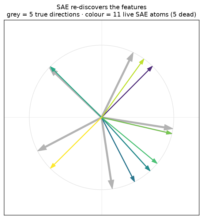
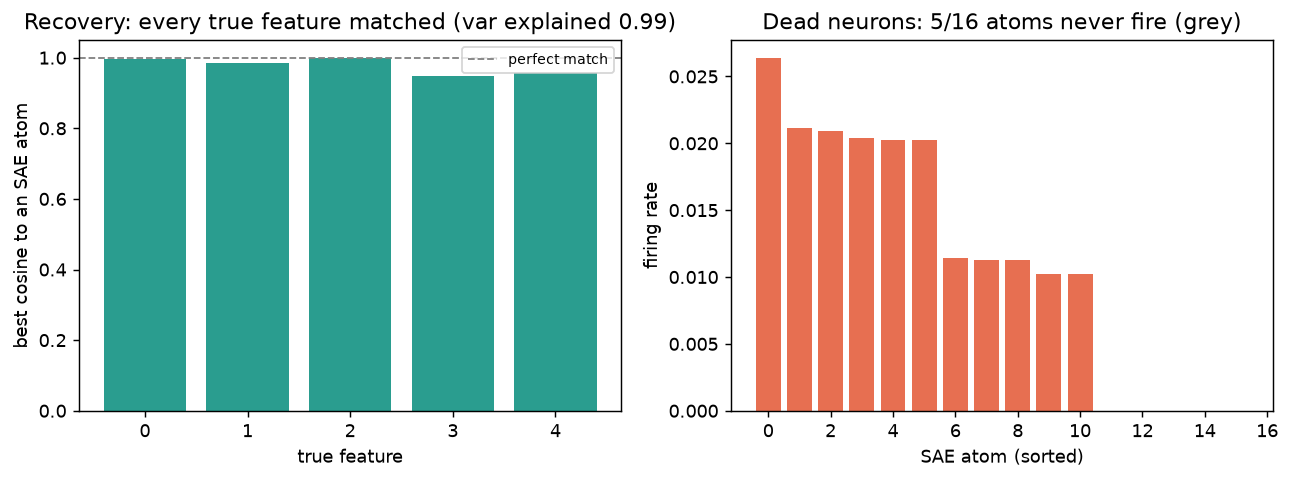
A sparse autoencoder (SAE) is the reverse move: instead of squeezing features into few dials, it spreads the tangled signal into a wide set of slots and forces only a few on at once. That pressure pushes each slot to become one clean feature. Because we invented the toy's features, we can grade it exactly.
go deeper — the sparsity trade-off
Sweeping the L1 sparsity penalty: raising it drops variance-explained 1.00 → 0.99 but lifts worst-feature recovery 0.74 → 0.93. Too little sparsity and two nearby features merge onto one slot; enough sparsity forces each example to use ~one slot, driving slots onto the true directions. Dead neurons and feature-splitting show up exactly as in real SAEs — a safe rehearsal for the real thing.
Real features, no answer key
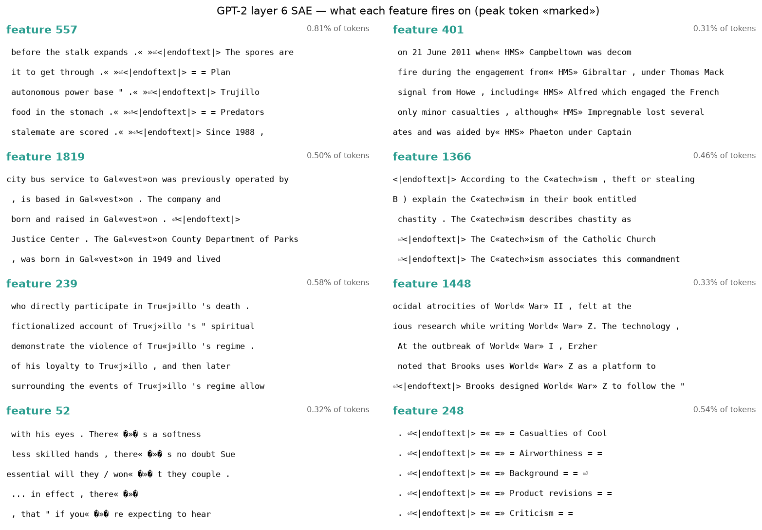
On a real model nobody knows the true features — so we judge a feature by the text that makes it fire. Train an SAE on ~480k GPT-2 activations and clean, single-meaning features fall out with no labels: one fires only on «HMS», one on «km» after a distance, one on the apostrophe in contractions.
go deeper — reading the health check
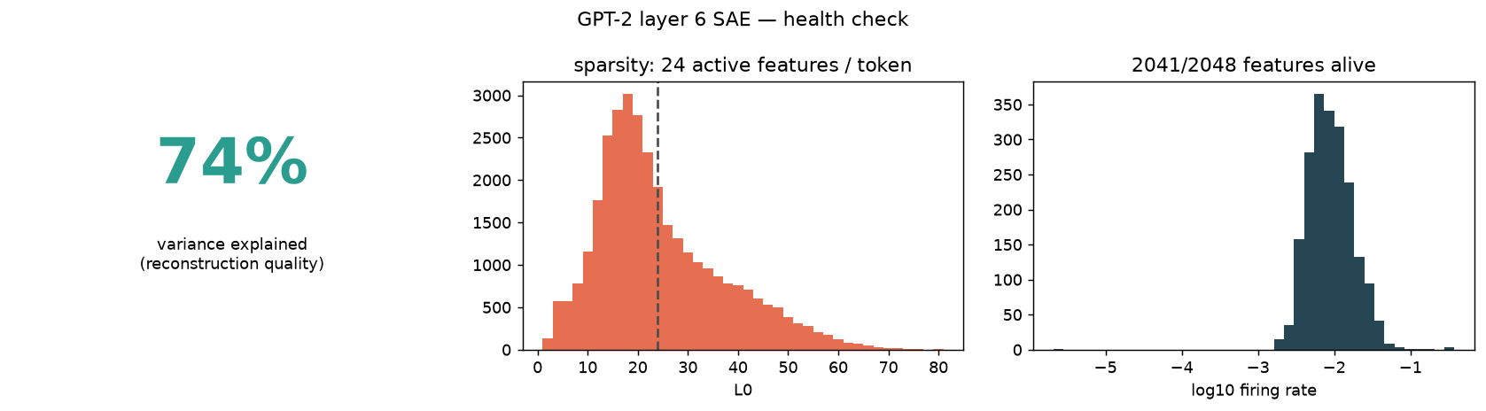
Same sparsity trade-off as tab 15, now on a real model: pushing from ~120 to ~24 active features per token drops reconstruction 85% → 74% but makes features far cleaner. A few features are boring corpus artifacts (Wikipedia's "= = Heading = =" formatting) — real SAEs always have a mix. 2041 of 2048 slots stay alive.
Grab a feature and steer
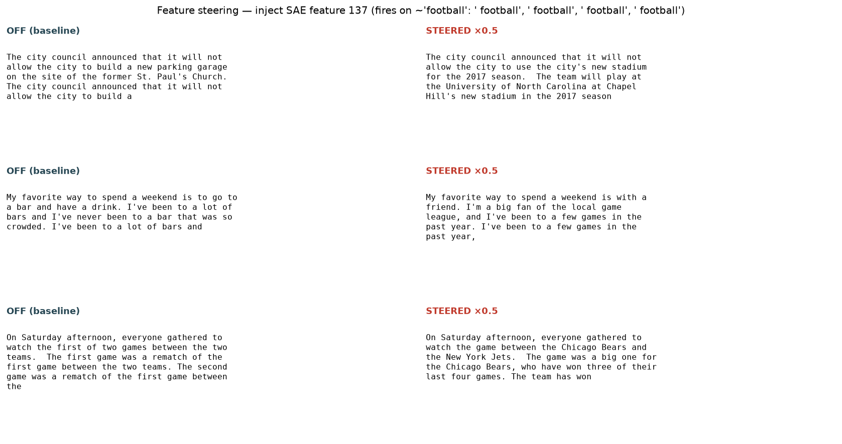
Reading a feature only shows correlation. The causal test: add it back in. Inject an SAE feature's direction into GPT-2 while it writes and watch the text bend to its concept — the same move as the refusal dial in tab 10, but the direction was found unsupervised.
go deeper — how the steering works
The SAE feature's decoder direction is added to the residual stream at every position during generation, scaled to a multiple of the feature's own peak activation. It's the exact intervention from tab 10 (add a direction, change the behaviour) — the only difference is that this direction was discovered automatically by the SAE instead of built from hand-labelled prompts. The same toolkit is how safety work detects and controls behaviours like refusal, deception, or bias.
Audit the dictionary — and find a hole in it
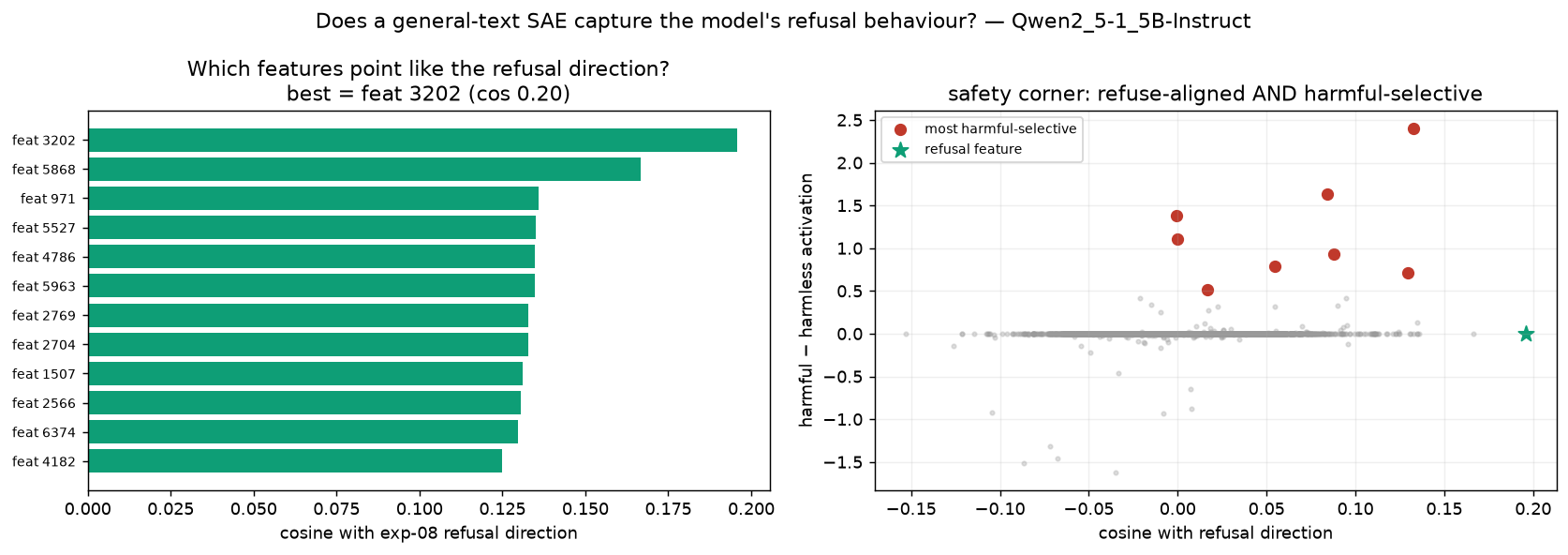
Tabs 14–17 built the SAE toolkit on GPT-2. Tab 10 built a safety tool on a chat model. Point the first at the second: train an SAE on the same model and same layer where tab 10 found the refusal direction, then search its dictionary for safety-relevant features.
Harmful topics show up cleanly — «nuclear», «gun», «attack», all firing on military history. That's worth saying carefully: these are knowledge features, not malice. A model needs a concept of "weapon" simply to refuse a weapon request.
go deeper — why "no feature found" is not "no feature exists"
This SAE was trained on Wikipedia. Wikipedia contains dangerous topics in abundance — but it contains no refusals, because nobody is asking Wikipedia for bomb instructions and being turned down. The behaviour was never in the training activations, so the SAE had no chance to build a feature for it. Tab 19 tests that explanation directly.
Change the diet, and the feature appears
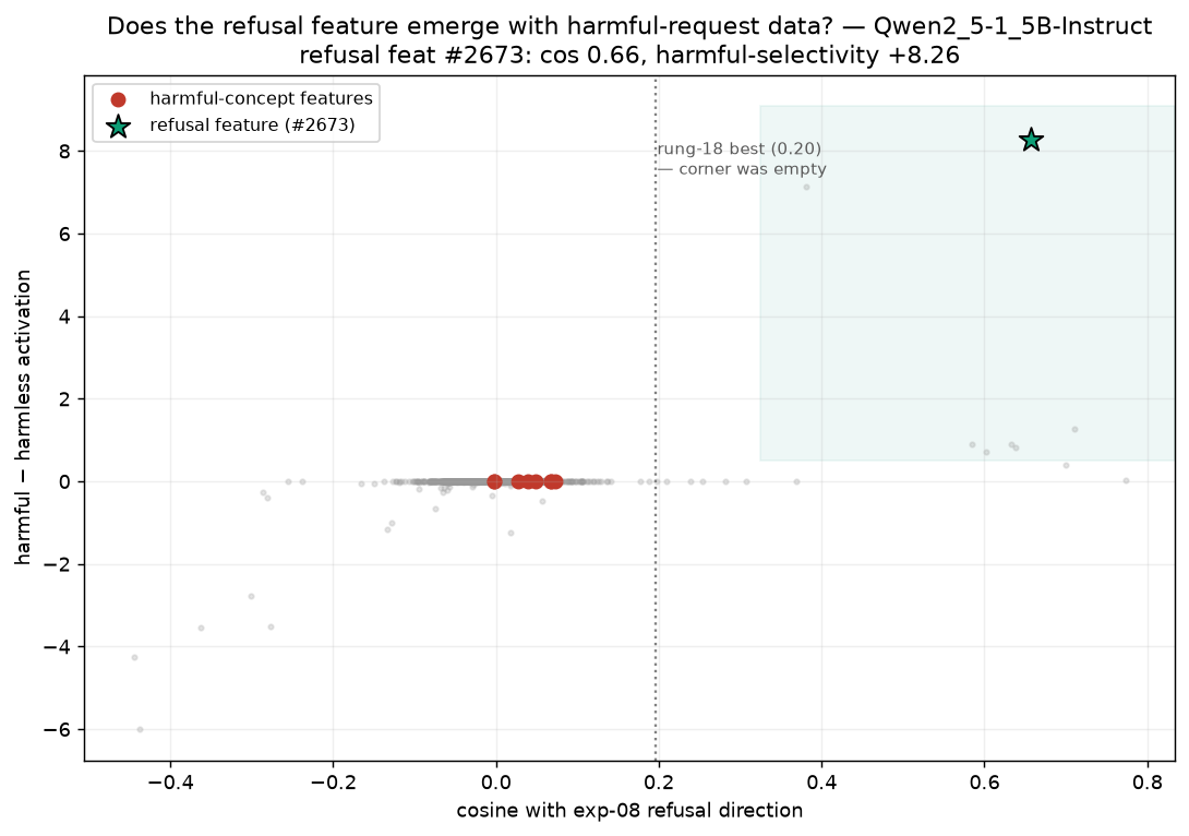
If the hole came from the data, changing the data should fill it. Same model, same layer, same SAE — but now it also sees the model's activations while it processes real harmful requests and benign ones, at the exact positions where the refuse-or-answer decision gets made.
go deeper — guarding against cheating (tab 19)
An obvious objection: if you train the SAE on the harmful prompts you're testing it with, of course it finds a "harmful feature" — it memorized them. So the harmful training requests (AdvBench) are kept disjoint from the harmful evaluation prompts, and the alignment score is measured against tab 10's direction, which was built independently. Feature #2673 is also the single most harmful-selective feature out of 4096 — but it isn't alone: about 7 features sit in that corner, a hint that refusal is spread across a small cluster rather than one atom.
Lever, or just a label?
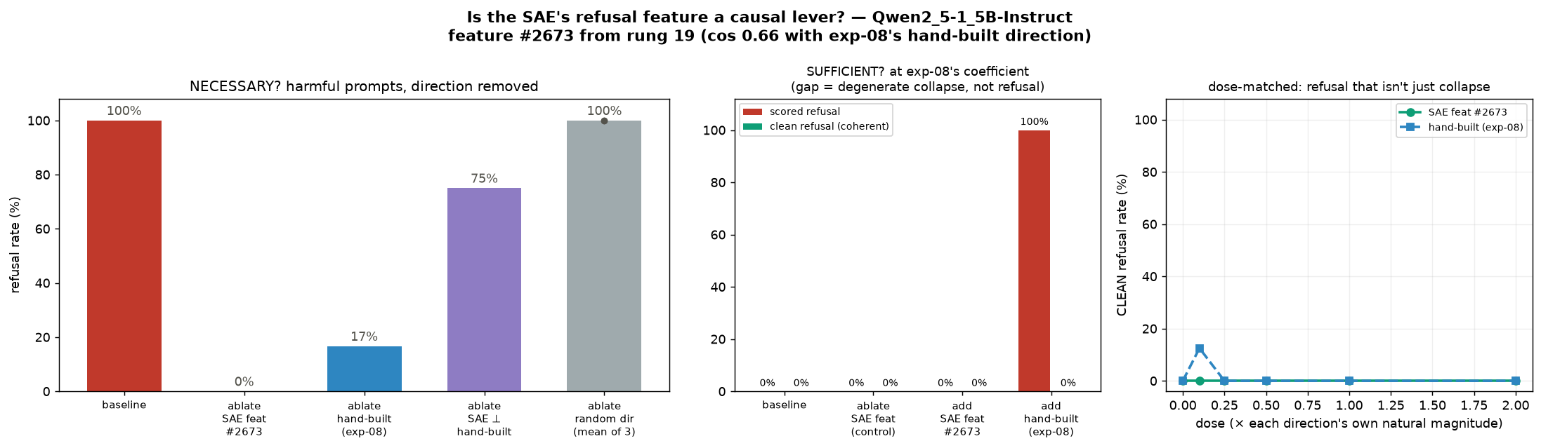
Everything in tab 19 was correlation: the feature lights up during refusals. A thermometer reads a fire without lighting it. So do what tab 17 did — intervene — but judged against the toughest benchmark available: the hand-built direction from tab 10 that we already know works.
go deeper — the two controls that made the difference
A coherence check. Every rate is now reported twice: "scored refusal" and "clean refusal" (refused and still writing varied text). The gap between the red and green bars in the middle panel is the artifact.
A dose-matched sweep. The first version of this experiment swept the injection strength upward (×1 → ×16) and got a flat zero — but tab 17 had already shown the usable range is around ×0.25–0.5, so that whole sweep sat inside the broken regime. Sweeping downward instead finds the honest answer: there is a window where the model still writes properly, and in it the SAE feature produces no refusal while the hand-built direction manages a narrow 12%.
One more clue that the SAE found something real: the part of the SAE feature pointing away from the hand-built direction still drops refusal to 75% by itself. The SAE didn't just re-discover the hand-built direction — it found refusal-relevant structure that averaging harmful-minus-harmless prompts misses.
Same story, different lab
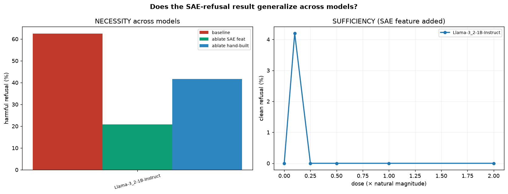
A fair objection to tabs 18–20: it's all one model. Maybe the empty corner, the diet effect and the ablation win are quirks of Qwen. So rerun the whole arc — audit, diet, causal test — on Llama-3.2-1B-Instruct: different company, different tokenizer, different architecture. All three findings replicate.
The audit (tab 18's move): a wikitext-only SAE on Llama has no refusal feature — best alignment with the hand-built direction is 0.199 (eerily close to Qwen's 0.196), and the safety corner is empty. The diet (tab 19's move): add harmful/benign chat activations and a refusal feature emerges — #2113, firing +19.9 harder on harmful prompts. One wrinkle: the corner now holds 2 features, each weaker-aligned than Qwen's single atom (0.40 vs 0.66) — in Llama, refusal smears across a small cluster.
go deeper — what changed across the lab line, and what didn't
The specifics are model-local: Llama's refusal direction sits at layer 11 of 16 (Qwen: 21 of 28), its feature is split over two weaker atoms, and its guardrails are thinner (62% baseline refusal vs Qwen's 100%). The structure is not: general-text SAE blind → diet fixes it → the SAE feature is the sharper scalpel. Even the sufficiency failure replicates in shape — hand-built 29%, SAE 4%, both only at the gentlest ×0.1 dose of an all-layers add (the next tab explains why that intervention was the real culprit). The run appends each model's numbers to a results JSON, so the chart is built to take a third and a fourth model on the same axes.
It was a switch all along
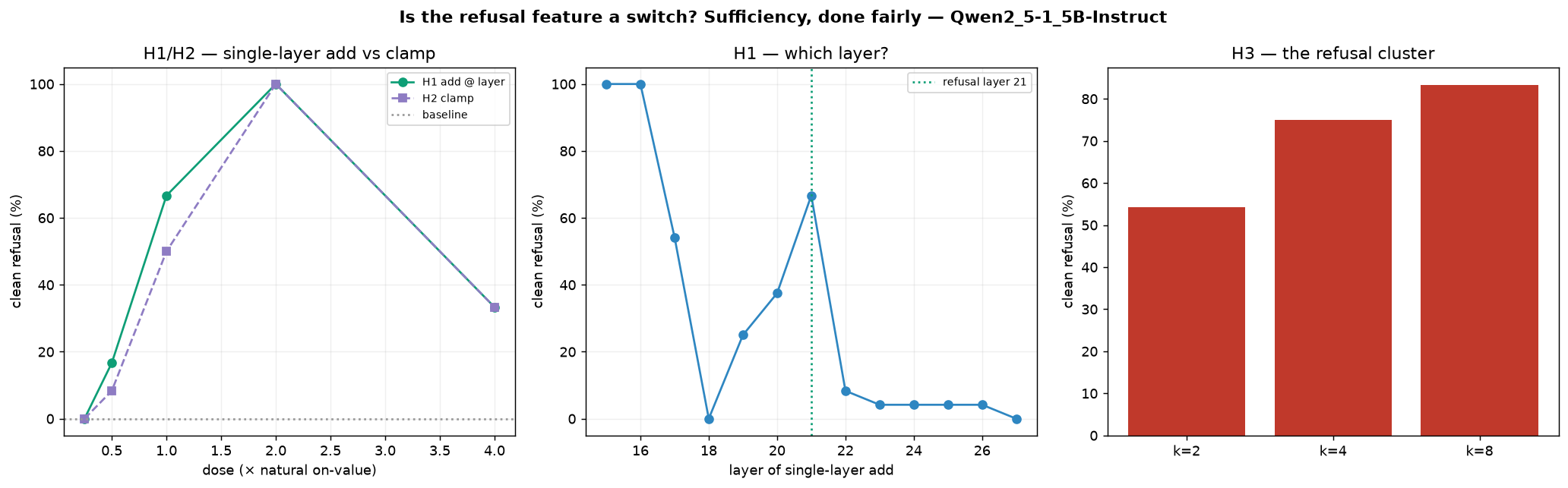
Tab 20's "necessary but not sufficient" had a suspect hiding in the method: it pushed the feature into all 28 layers at once. This experiment separates the feature from the injection — three hypotheses, each a fairer version of "turn it on." The feature was fine. The injection was the problem.
First, reproduce the failure: add at every layer at ×1 → 0% refusal, exactly as tab 20 found. Now add at one layer — the layer the feature came from — and sweep the dose ×0.25 → ×4: clean refusal goes 0% → 17% → 67% → 100% → 33%, with zero degenerate output at every dose. A textbook dose-response, honest inverted-U included — over-dose and refusal declines, but the model stays coherent. At ×2 it politely refuses to explain how to make a paper airplane.
go deeper — the three hypotheses, scored
H1 — wrong site? Yes. All-layers add: 0%. Single-layer add at layer 21: 100% at ×2. Sweeping the injection layer (add ×1 at each of L15…L27) finds a clean window: L15–16 perfect, L17–20 refusing but increasingly breaking the model (L18: 100% degenerate), L22 onward inert — the refusal decision has already been read out of the stream by then.
H2 — wrong magnitude semantics? No. Clamping the feature to its natural on-value through the SAE encoder — the SAE-native way to say "this feature is on" — tracks the raw add curve almost exactly and also hits 100% at ×2. So it was never about how much; only where.
H3 — needs the whole cluster? No. Clamping the top-2 / 4 / 8 refusal-cluster features together at ×1 each gives 54% / 75% / 83% — the cluster helps at gentle doses, but one feature at ×2 already closes the case.
Housekeeping: the refusal-diet SAE was retrained for this experiment, so its feature id is #923 (alignment 0.62, harmful-selectivity +18.2) rather than tab 19's #2673 — SAE training isn't deterministic, but the same search finds the same feature. And "clean refusal" everywhere above means refused and coherent: tab 20's control, kept on.
Features grow wires
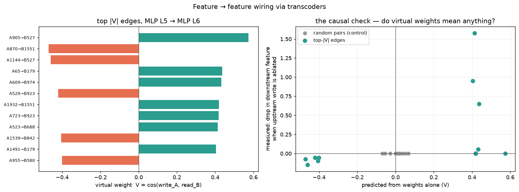
An SAE feature is a point: it says a concept exists, not where it comes from or where it goes. A transcoder is the same sparse dictionary trained to imitate what an MLP layer computes instead of copying its input — so every feature gets two directions: a read (what makes it fire) and a write (what it adds back to the stream). Suddenly "does feature A feed feature B?" is arithmetic: line A's write up against B's read.
Train one on GPT-2's layer-5 MLP and one on layer 6 (tab 16's data and recipe) and the features come out just as crisply single-meaning as tab 16's — «Year» inside award names, the «myel-» medical morpheme, dollar amounts, contractions — with several concepts recurring at both layers. Then the new trick: for every cross-layer feature pair, a virtual weight — how well A's write lines up with B's read — predicts the wiring from weights alone, before running the model at all.
go deeper — why a transcoder scores "worse" than an SAE
The health check reads 47% variance explained per transcoder, against the tab-16 SAE's 74% — and that's correct, not a failure: an SAE only has to copy its own input, while a transcoder must predict what a whole MLP layer computes from it, a strictly harder job. Sparsity and coverage stay healthy (~16 features active per token, ~2040 of 2048 alive). And the number to watch was never reconstruction anyway — tab 15 made that point — it's whether the features are real, and the sign-matched ablations say they are.
Who writes the refusal signal?
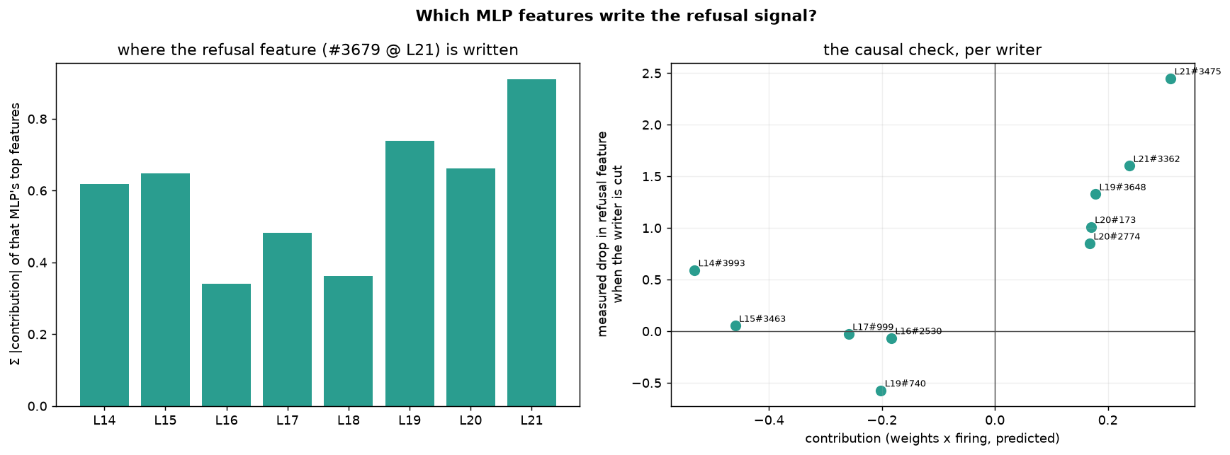
Tab 22 left an X on the map: inject at L15–16, read out at L21 — something in between turns "this request is harmful" into "refuse." Now there's a tool to ask directly. Re-find the refusal feature with tab 19's diet SAE, train a transcoder at every MLP in that window (L14–L21), and score every feature: its write's alignment with the refusal feature's read, times how hard it fires on harmful requests — tab 23's zero-edge lesson, applied.
The writers that survive the causal check are all last-token harmful-request detectors at layers 19–21 — features that fire on "make a bomb" / "spread malware" prompts. Cutting any one drops the refusal feature by 0.85–2.45 of its 21.4 baseline, with layer 21's own MLP the biggest single writer. And one genuine inhibitor validates: an L19 feature that fires on ordinary task requests, whose removal raises the refusal feature — a "this is a normal request" wire actively holding refusal down.
go deeper — why the feature id keeps changing
This training of the diet SAE finds the refusal feature as #3679 (alignment 0.45 with the hand-built direction) — tab 19 said #2673, tab 22 said #923. SAE training isn't deterministic, so the id and exact alignment change every retraining; what's stable is that the same search (refusal-aligned and harmful-selective) keeps finding the same feature. The contribution score here is cos(write, read) × firing on harmful requests — the activation weighting is what tab 23's zero-effect edges taught: alignment alone counts wiring the data never uses.
Attribution graphs on a desktop GPU
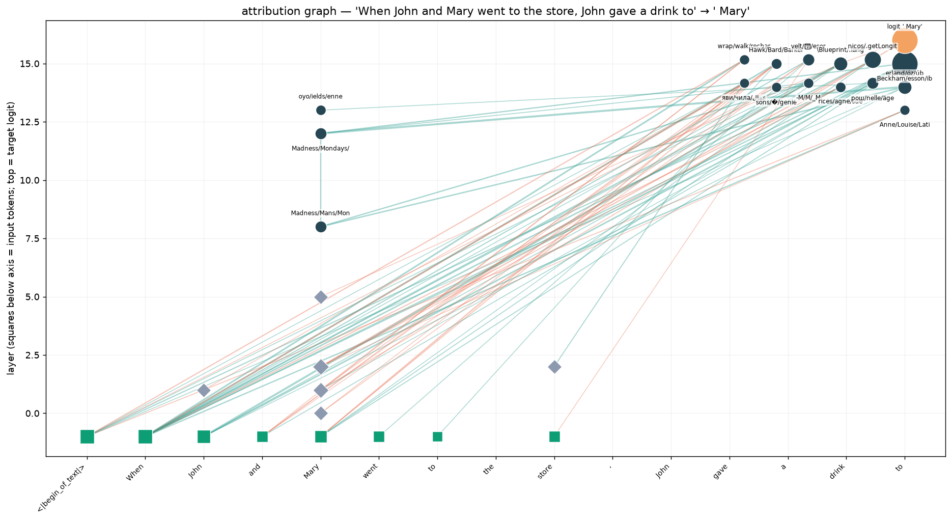
Tabs 23–24 measured exactly where one-hop wiring breaks: aligned edges that never co-fire, and cosines that stop predicting across four blocks. The attribution graph is the tool built for both: freeze a real forward pass's attention patterns and LayerNorms, swap every MLP for a transcoder, then back-propagate influence from one chosen output token through every feature at every position — multi-hop, attention-routed, position-resolved.
This runs Anthropic's open-source circuit-tracer with a community transcoder set for Llama-3.2-1B — 16 layers × 131k features, ~17 GB of weights — on the same 12 GB desktop GPU as everything else in this repo. Two canonical circuits: dallas ("the capital of the state containing Dallas is" → traced toward " Austin"), whose graph carries «capital/capitals», «Missouri/Iowa/Wisconsin» and «Texas/TX» features feeding a late-layer cluster at the answer position; and ioi ("When John and Mary went to the store, John gave a drink to" → " Mary", the model's genuine top pick), which shows the classic name-mover shape.
go deeper — two honesty wrinkles
The model doesn't actually say Austin. Tiny Llama's top prediction for the dallas prompt is a prompt-echo " Dallas" at 13% — " Austin" sits at rank 5 with 5%. The graph is traced toward the Austin logit explicitly, which is legitimate (attribution asks "what pushes this output up?", whatever its rank) — but a writeup that hid the echo would be dressing a 1B model up as Claude. Kept, on purpose.
Feature labels are cheap. Each node's name comes from a quick logit-lens readout — crisp for token-ish features («Texas/TX»), muddy for abstract ones. The graph's structure is measured; the words on the nodes are best-effort glosses, not ground truth.